The global climate accelerator and the financial accelerator: Clarifying the commonalities, and implications from Putin’s war

Scientists fear for the climate. Tipping points Lenton et. al. 2019, IPCC 2021, and 2022). The global climate accelerator is a phenomenon in which an accumulation of greenhouse gases leads to higher global temperatures and more carbon, eventually making the planet uninhabitable. We are facing a climate change KriseThe world is dangerously close at the tipping points where irreversible changes could occur. Both the global climate accelerator and the financial accelerator (for example, during the Global Financial Crisis (GFC),) are characterised by highly nonlinear feedback loops. The GFC saw falling real estate prices amplified by the financial system, and its interaction with the real world, which led to further price declines. The GFC and Great Depression had similar financial crises. They were characterized by falling stock markets, bankruptcies and foreclosures of many homes. 

They share a commonality in that lobbying and special interest corrupt financial regulation and climate regulation. This helps spread harmful distortions of the facts. Common is the fact that the GFC and global carbon emission have been caused by the richest countries (Chancel, Piketty 2015). 

There are also important differences. There is a floor to real property prices even without intervention from policy. This is because housing demand eventually responds to lower prices. But, without policy intervention there is no natural ceiling on global temperatures that is consistent with reasonable survival prospects. A second difference concerns different time scales – mere months for the financial accelerator, but decades and eventually millennia for the climate accelerator, given the PersistenceThe stock of greenhouse gases. This time frame makes it impossible for policymakers to be too optimistic about climate action. A third difference is that, in the GFC, the financial accelerator’s effects were concentrated in affluent financialised countries. The climate accelerator has global consequences, and will have a severe impact on many poor countries over the medium-term (Cruz & Rossi-Hansberg, 2021). 

It is now well-known that the links between global economy and financial system were not well understood during the GFC. These non-linear phenomena are still not well understood and need to be addressed urgently. Analogous issues also apply to climate models created by economists: they need to similarly include non-linearities that are related to climate and financial. Policymakers require a qualitative understanding of these dual nonlinearities, even if they don’t have detailed models. This column identifies the similarities between these processes for the climate as well as financial accelerators.

The GFC, and its aftermath, diverted attention from important mitigation strategies, delaying necessary climate change action. Pre-GFC, the IMF wrote: “Climate change is a potentially catastrophic global externality and one of the world’s greatest collective action problems…The costs of policies to address climate change can be contained by ensuring that mitigation policies are well designed. It is crucial to create a framework that is sustainable, and encourages broad participation from all countries.” (IMF 2008). However, fiscal capacity for ‘greening’ was severely curtailed. Bankers, who were rescued at great cost, kept their pensions and bonuses. The majority of the population experienced high unemployment, loss in income, and sometimes lost their homes. The reputational damage to politicians and policymakers fueled the rise in libertarian or nationalistic populism. This limited the ability to take collective action to address climate issues. 

The effect of Russia’s war on climate and in delaying climate action are serious and it presents risks to global financial stability. Policymakers should be able to understand the nature of climate and financial accelerators, as well as their longer-term links, in order to address the new risks and challenges posed by the war.

The global climate accelerator 

The global climate system is affected by amplifying feedback. The rise in temperatures from the accumulation of greenhouse gases – through burning fossil fuels, and the release of methane incidental to extraction of oil and natural gas and via intensive livestock farming – itself causes further temperature rises and further carbon emissions. Table 1 lists the mechanisms that increase the chance of irreversible climate shifts when certain tipping points have been breached. Worse equilibrium state may lead to mass species extinction and major sea-level rises. 2019, IPCC 2021, United Nations Environment Programme 2021). Table 1 shows that there are very few stabilizing or offsetting processes at a relevant scale. Each IPCC report paints an even more alarming picture of the dangers facing us. Figure 1 shows the alarming rise in global average temperatures caused by man.  

Table 1Transmission and amplification in the global climate system

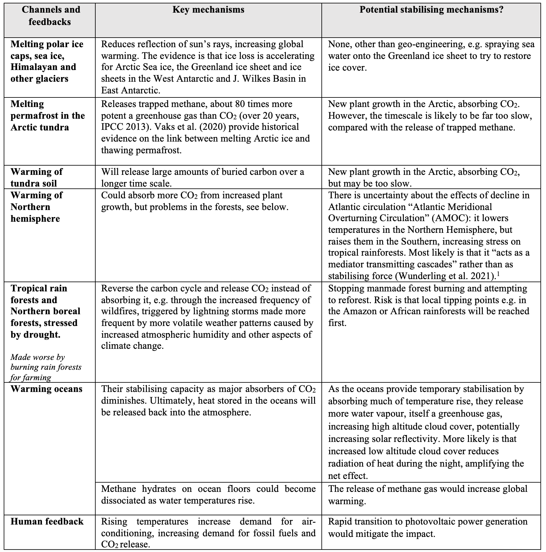
Figure 1 Rising global temperatures. 

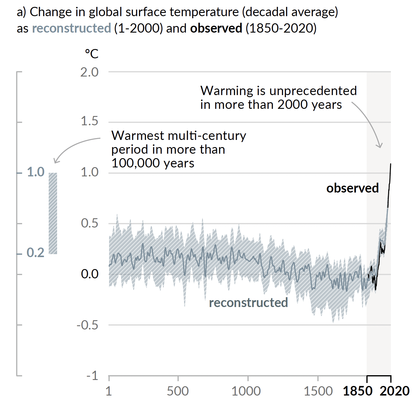
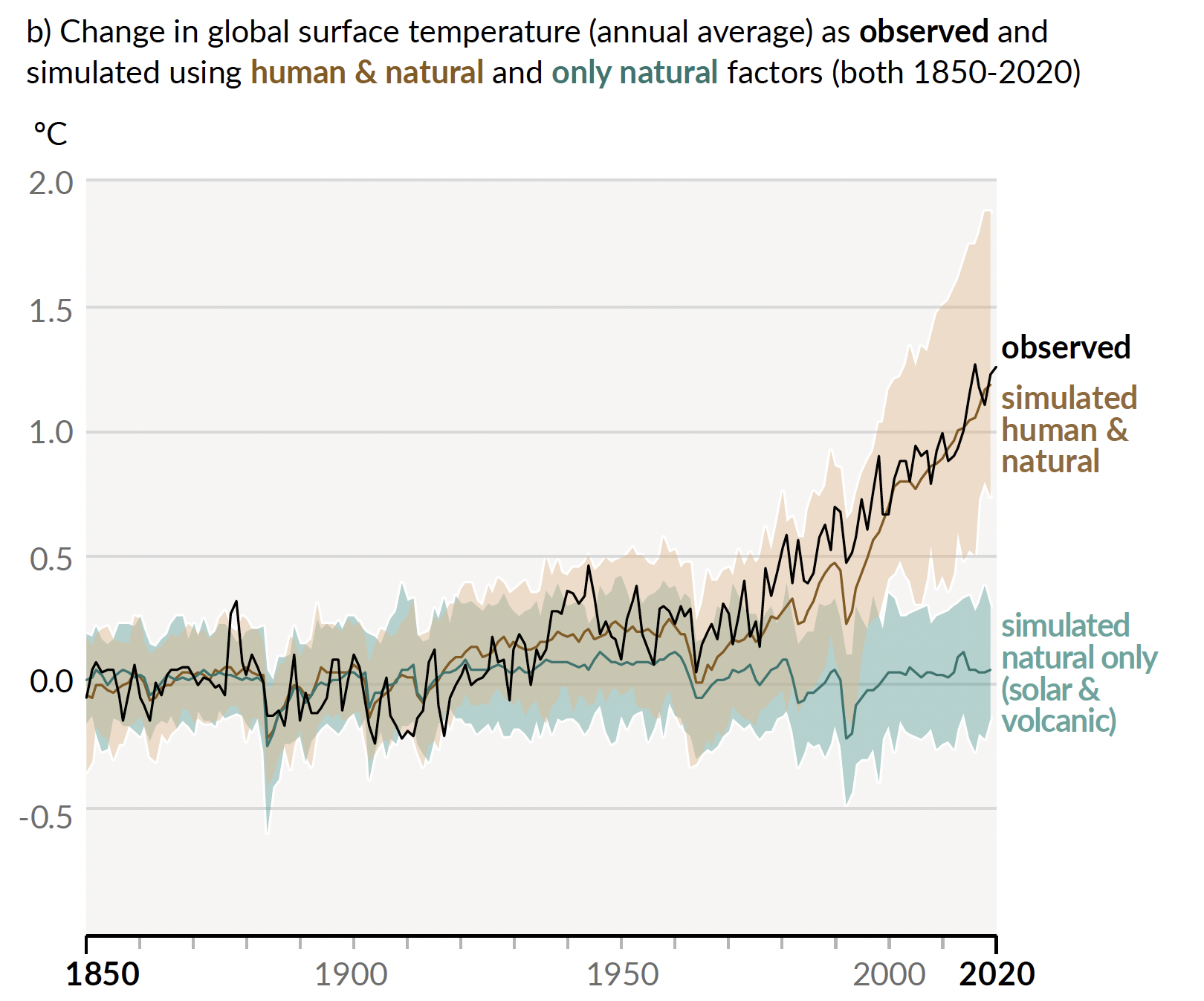
SourceIPCC (2021), Figure SPM.1.

The GFC’s financial accelerator

Recent research on international house prices cycles has revealed a complex system of interactions between real economy and financial sector. These interactions operate in both directions. Figure 2 shows how a negative shock could affect US house prices during a sub-prime crisis. The shocks were severe Amplifiedimportant non-linearities. 

Figure 2’s left side shows how falling house prices are transmitted to the real world and back to houses prices. Figure 2’s right side shows how they are transmitted to the financial sector. The interactions between sectors is indicated. The four sideways transmission signs in the bottom right-hand corner represent the interactions between sectors.The impact of credit conditionsThe real economy components of construction, real estate demand, and consumption are all linked to GDP. Thin upward arrows show the feedback channels between real components and house prices. House price shocks can be amplified within the financial system (through contagion), and between the real economy and the financial sector. 

Figure 2The financial accelerator (example: the US subprime crisis).

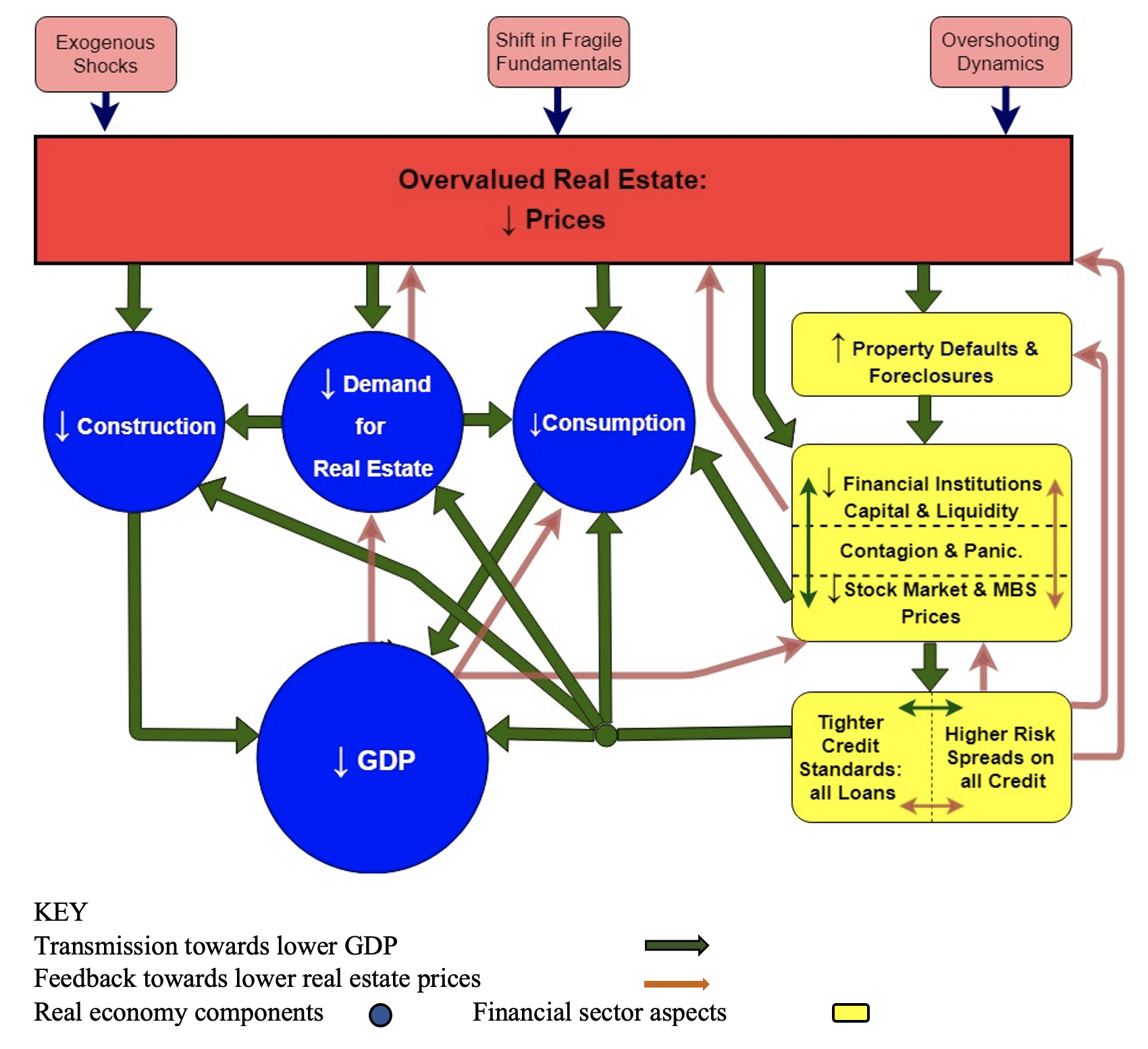
Source: Duca et al. (2021). 

The US crisis began when an overvalued realty sector collapsed due to weak financial fundamentals. Due to two deregulations, the system was too heavily leveraged with poor lending quality.² Homebuyers extrapolated the observed strong house price gains, driven by deregulation and by positive economic news, so that house prices became increasingly overvalued just as households’ rising debt levels made them more vulnerable. 

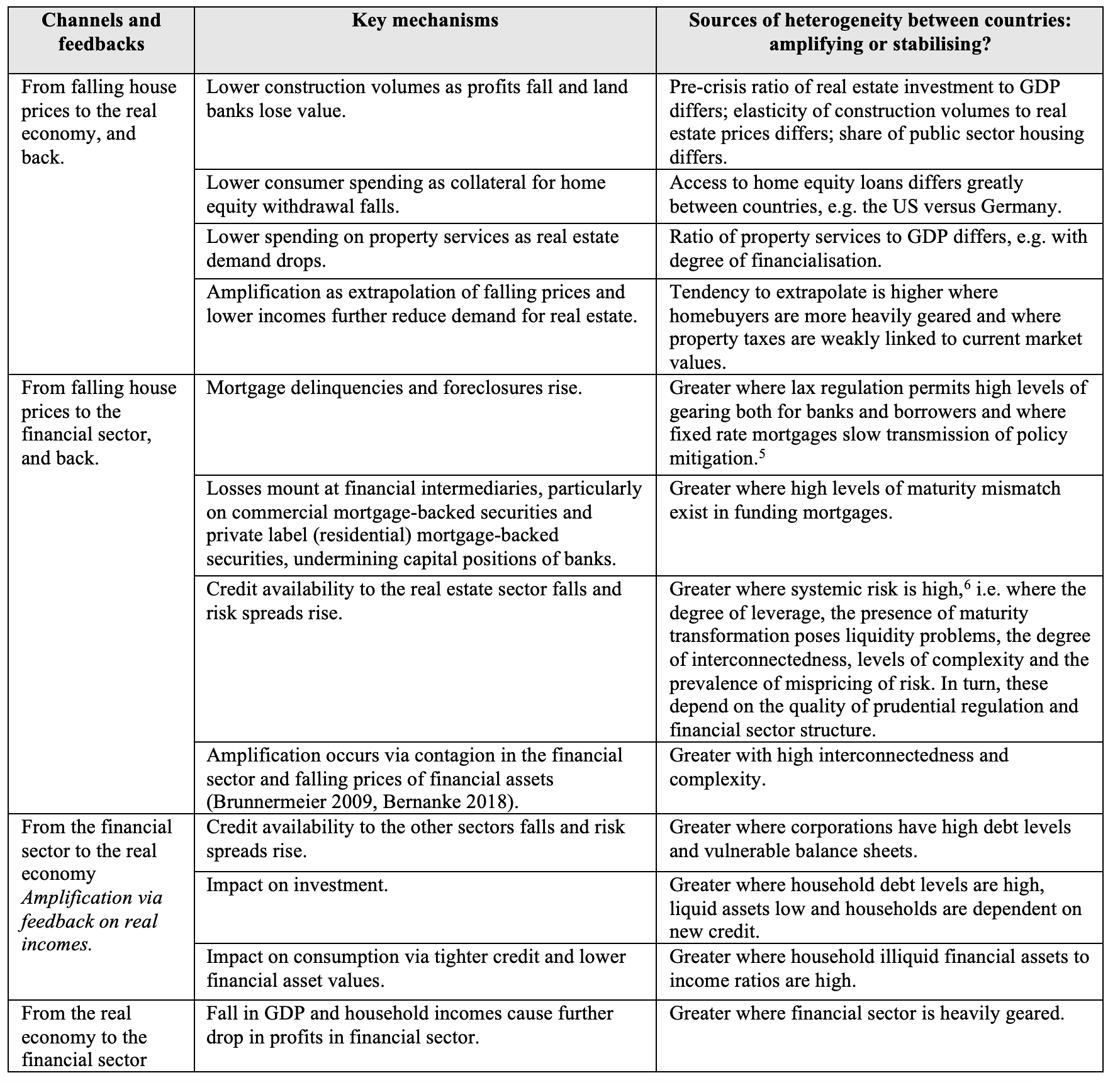
Duca et al. provide a detailed discussion of the channels and feedbacks as well as potential amplification. (2021).³ A summary of the mechanisms in the financial accelerator in the US in the GFC is given in Table 2. This table also shows how differences between countries and regulation can affect the transmission and the degree to which amplification occurs. The table contains a lot of micro- and macro evidence for the connections between consumption and house price.⁴  

Table 2 Transmission and amplification of a negative house-price shock in the GFC

Weaknesses in economic policies models during and after GFC

The New Keynesian dynamic stochastic global equilibrium (NK-DSGE), models that governed macroeconomic policymaking and thinking prior to the GFC failed completely during the crisis. They were based upon linear reasoning and assumed a stable long-run equilibrium. They failed to recognize coordination failures, particularly between finance and the real economy, and were therefore not able to understand financial stability. They were insufficiently ‘dynamic’ and misled on real-world lag structures. They were hardly ‘stochastic’, since they lacked, for probability distributions, both radical uncertainty (the time dimension) and heterogeneity (the cross-section dimension) (Muellbauer 2010, 2018). Radical uncertainty is endemic due to the possibility of non-linearities or structural breaks. This undermines the relevance of key assumptions of NK-DSGE models – ‘rational’ expectations and inter-temporal optimisation which hold that all economic agents share knowledge of the same stable model of the economy (Hendry and Mizon 2014).

Post-GFC, central banks have placed more reliance on semi-structural models, such as the Federal Reserve’s FRB-US, based on less unrealistic assumptions and with greater scope for the data to ‘speak’. However, the household sector of these models is still lacking the transmission channels for credit shifts or house prices (Muellbauer 2020).⁷  

Weaknesses in economic model that attempts to integrate climate 

Oswald and Stern (2019) argue that, on climate change, “academic economists are letting down the world”,⁸ with most top journals ignoring or mis-representing the issue.

Franta (2021), analyzes the harmful role of an influential group economic consultants, hired from the fossil fuel industry in the 1990s to 2010 to estimate the costs associated with various climate policies.⁹ He argues that their work “played a key role in undermining numerous major climate policy initiatives in the US over a span of decades, including carbon pricing and participation in international climate agreements”. This unfortunately influenced the conservative assumptions used for integrated assessment models (IAMs), that attempt to integrate climate science and economic models for cost/benefit analysis and computation of the social cost. Nordhaus 1991, 1992). The output from IAM models is governed primarily by two assumptions: social discount rateThe Climate sensitivity of GDP (i.e. (Pindyck 2017)  If a low discount rate of 3% is assumed and a linear relationship between temperature and GDP, then even a 5°C rise in global average temperatures will have only a moderate impact on GDP. The social cost of carbon is estimated at $11 (Nordhaus 2011, p. Stern (2007) estimated that this figure was over $200. Stern (2013) stresses that many IAMs are guilty of underestimating or ignoring the potential for catastrophic outcomes due to the non-linearity of the global climate accelerator. To accurately estimate the social costs of carbon, it is important to include people.

Other problems with IAMs mirror the economic policy models. These include the exclusion of interaction effects¹⁰ and radical uncertainty, and the assumption of rational (model-consistent) expectations and representative agents when there is much heterogeneity in practice (Farmer et al. 2015, Hepburn, Farmer 2020. Asefi Najafabady and al. 2021). Many IAMs ignore feedbacks between climate change and human systems, except in trivial cases.¹¹ 

It was late for central banks to address the effects of climate change upon financial stability. In 2017, the Network for Greening the Financial System (NGFS) was launched. 108 central banks and regulators now belong to the network. Financial stability will be affected by both transition and physical risks to assets and properties from climate change and the income-reducing effects of disruptions in trade and production. These risks are assessed using climate stress tests. The adjustments include disclosure requirements, guidance, new risk weights or capital requirements, as well as alignment of monetary policy instruments (e.g. adjusting ‘haircuts’ on collateral for climate risk) (Loyttyniemi 2021, Network for Greening the Financial System 2019, Bolton et al. 2020).¹² Central banks have begun incorporating climate features into macroeconomic models (ECB 2021), and some of these model developments will prove relevant in current forecasting and policy simulation.

Implications of Russia’s war for financial stability and the climate

Central banks are now better placed to address the risks to financial stability generated by Russia’s war on Ukraine. Monitoring financial stability and prudential regulations does not rely too heavily upon the current generation of inept policy models. This has significantly improved since the GFC. Risks include a new sovereign debt crisis given the downgrade or default of Russia’s foreign-currency debt, much of it held in Europe. A credit crunch could follow the spillover effects of falls in asset values from Russian companies that have invested in Russian assets. 

The war’s effects on the Earth’s climate are potentially even more serious. The reconstruction of the cities that were destroyed in Ukraine could have significant climate consequences. The construction phase is responsible for between 30% and 70% of the building’s lifetime carbon emissions (e.g. OECD 2021 and Arup 2022). Retrofitting existing buildings is generally a better strategy than demolition and reconstruction. Putin’s war machine is achieving the exact opposite, and at a staggering human cost. The rush to increase oil and gas production with energy security likely to dominate climate issues for years to come could delay the greening the global economy by many years. While it will increase green investments over the longer term and encourage the development and adoption green technologies, the danger of a delay in now is heightened by the proximity to tipping points within the global climate system.

Author’s note: We are grateful to David Hendry, Cameron Hepburn, Francois Lafond, Avner Offer, Ryan Raferty and Dennis Snower for their input, but take responsibility for errors.

Refer to

Adrian, T, D M Covitz, and N Liang (2015), “Financial stability monitoring”, Annual Review of Financial Economics 7: 357-395. 

Andersen, A L, C Duus and T L Jensen (2016), “Household debt and spending during the financial crisis: Evidence from Danish micro data”, European Economic Review 89: 96-115.

Aron, J, J V Duca, J Muellbauer, A Murphy, and K Murata (2012), ““Evidence from the U.K. and Japan on credit, housing collateral, and consumption“, Review of Income & Wealth 58 (3): 397-423.

Arup (2022), “How to reduce your carbon emissions”, online.

Asefi-Najafabady, S, L Villegas-Ortiz, and J Morgan (2021), “The failure of Integrated Assessment Models as a response to ‘climate emergency’ and ecological breakdown: The emperor has no clothes”, Globalization 18(7): 1178-1188.

Berger, D, V Guerrieri, G Lorenzoni, and J Vavra (2018), “House prices and consumer spending”, Review of Economic Studies 85(3): 1502–42.

Bernanke, B (2018), “The real effects of disrupted credit: Evidence from the global financial crisis”, Brookings Papers on Economic Activity, September.

Bolton, P. D Morgan L A Pereira da Silva F Samama R Svartzman 2020 The green swan – Central banking and financial stability in an age of climate changes Basel, Switzerland: Bank for International Settlements. 

Browning, M, M Gortz, and S Leth-Petersen( 2013), “Housing wealth and consumption: A micro panel study”, The Economic Journal 123: 401–28.

Brunnermeier, M K (2009), “Understanding the liquidity and credit crunch 2007–2008“, Journal of Economic Perspectives 23 (1): 77-100. 

Calza, A, T Monacelli, and L Stracca (2013), “Housing finance and monetary policy”, Journal of the European Economic Association 11(suppl_1, 1): 101–22.

Castle JL and D F Hendry (2020),Climate econometrics: An overview“,Econometrics Trends and Foundations 10 (3-4): 145-322. 

Chancel, L and T Piketty (2015), “Carbon and inequality: Kyoto to Paris”, VoxEU.org, 01 December.

Chauvin, V and J Muellbauer (2018), “France: Consumption, household portfolios, and the housing market”, Economie et Statistique/Economics and Statistics 500-501-502: 157-178. 

Cruz, J-L and E Rossi-Hansberg (2021), “Uneven gains: Assessing the global warming’s economic impact on the economy in aggregate and in a spatial context”, VoxEU.org, 2 March.

Duca, J V, J Muellbauer, and A Murphy (2021), “What drives house-price cycles? International experience and policy issues”, Journal of Economic Literature 59(3): 773-864.

ECB (2021), “Climate change and monetary Policy in the Euro Area”, ECB Strategic Review, Occasional paper series 271, September.

Farmer, J, C Hepburn, P Mealy, and A Teytelboym (2015), “A third wave in economics and climate change”, Environmental & Resource Economics 62 (2): 329-357. 

Franta, B (2021), “Weaponizing economics: Big Oil and economic consultants. Climate policy delay”, Environmental Politics, DOI: 10.1080/09644016.2021.1947636 

Geiger, F, J Muellbauer, and M Rupprecht (2016), “The German consumer, household portfolios, and the housing market”, European Central Bank Working Paper Series 1904.

Hendry, D F (2014), “Climate change: Lessons from our distant past”, VoxEU.org, 27 October.

Hendry, D F and G Mizon (2014), “Why standard macro-models fail when faced with crises”, VoxEU.org, 18 June.

Hepburn, C and J D Farmer (2020), “Less precision, more truth: uncertainty in climate economics and macroprudential policy”, in G Chichilnisky and A Rezai (eds), Handbook on the Economics of Climate Change, 420-438, Cheltenham: Edward Elgar Publishing.

Hurst, E and F Stafford (2004), “Equity is at home: Mortgage refinancing and household use”, Journal of Money, Credit and Banking 36(6): 985–1014.

IMF (2008) The business cycle and housing, April, World Economic Outlook. 

IPCC (2021), “Crushing climate impacts to hit sooner than feared”, AR6 Climate Change 2021 – The Physical Science Basis,UN: Intergovernmental Panel on Climate Change

IPCC (2022), “Climate change: A threat to human wellbeing and health of the planet”, United Nations: Intergovernmental Panel on Climate Change.

Lenton, T M, J Rockstrom, O Gaffney, S Rahmstorf, K Richardson, W Steffen, and H J  Schellnuber (2020), “Climate tipping points are too risky to bet against”, Nature 575(7784): 592–595.

Loyttyniemi, T (2021), “Incorporating climate change into the financial stability framework”, VoxEU.org, 8 July.

Mian, A and A Sufi (2014), ‘”House price increases and U.S. household spending between 2002 and 2006”, NBER Working Paper No. 20152. 

Mian, A and A Sufi (2018), “Finance and business cycles – The credit driven household demand channel,” Journal of Economic Perspectives 32(3): 31–58.

Mishkin, F (2007), “Housing and the monetary transmission mechanism”, in Housing, Housing Finance, and Monetary Policy. Proceedings of the Economic Policy SymposiumFederal Reserve Bank of Kansas City Jackson Hole Wyoming, 359-413.

Muellbauer, J (2010), “Designing central bank models: implications for household decisions, credit markets and macroeconomy”, Bank for International Settlements, discussion paper 306, March. 

Muellbauer, J (2018), “The future of macroeconomics”, The future of central banking: Festschrift in honour of Vítor Constâncio, ECB, December, 6-46.

Muellbauer, J (2020), “Implications for household-level evidence in policy models: The example of macro-financial linkingages“, Oxford Review of Economic Policy 36(3): 510-555.

Network for Greening the Financial System (2019), “First comprehensive report: A call to action on climate change as a source financial risk”, NGFS: Banque de France.

Nordhaus, W (1991), “To slow or not to slow: The economics of the greenhouse effect”, Economic Journal 101(407): 920–937. 

Nordhaus, W (1992), “An optimal transition path for controlling greenhouse gases”, Science 258(5086): 1315–1319.

Nordhaus, W (2011), “Estimates of the social cost of carbon: Background and results from the RICE-2011 model”, NBER Working Paper 17540.

OECD (2021), Brick by brick: Building better policies for housing, Paris: OECD.

Oswald, A and N Stern (2019), “Why are economists failing to see the importance of climate change in the world?”, VoxEU.org, 17 September.

Pindyck, R (2017) “Models for climate policy: Use and misuse”, Review of Environmental Economics and Policy 11(1): 100114. 

Stavins, R (2019), “Martin Weitzman’s contributions to environmental economics are a gift that keeps giving:”, VoxEU.org, 9 September.

Stern, N (2007).The Stern review: The economics of climate ChangeCambridge University Press.

Stern, N (2013), “The structure of economic modelling of potential climate change effects: Grafting gross underestimates of risk onto already narrow science models”, Journal of Economic Literature 51(3): 838–59.

Stout, L.A (2011), “Derivatives & the legal origins of the 2008 credit crises”. Harvard Business Law Review 1(1): 1–38. 

United Nations Environment Programme (2021), Emissions gap report 2021: The heat is on – A world of climate promises not yet delivered, Nairobi.

Vaks, A, A J Mason, S F M Breitenbach, A M Kononov, A V Osinzev, M Rosensaft, A Borshevsky, O S Gutareva, and G M Henderson (2020), “Evidence from paleoclimate that vulnerable permafrost is present during low sea ice”, Nature 577: 221–225.

Windsor, C, J P Jääskelä, and R Finlay (2015), “Housing wealth effects: Evidence from an Australian panel”, Economica 82: 552-577.

Wunderling, N, J F Donges, J Kurths, and R Winkelmann (2021), “Interacting tipping elements increase risk of climate domino effects under global warming”, Earth System Dynamics 12: 601–619.

Endnotes

1 However, Wunderling et al. did not include melting permafrost (Vaks et al. 2020) among their possible interactions, so underestimate the risks.

2 The Commodity Futures Modernization Act (2000) prioritised financial derivatives ahead of other debt claims, made enforceable throughout the US. Private issuers of mortgage-backed securities were encouraged by the government to use derivatives to reduce risk (Stout 2011,). These derivatives were used to create the illusion that low-quality mortgage-backed loans were investment grade due to their widespread use in deepening secondary market. Another deregulation measure was the 2004 Securities and Exchange Commission decision to relax capital requirements for investment banks. This caused a dangerous increase in gearing.

3 In addition to contagion within the financial system, a second important non-linearity occurred because a given house price fall results in a far larger increase in bad loans and hence credit contraction, if it follows a preceding fall. The third large nonlinearity resulted from tighter credit conditions amplifying the decline of housing collateral for consumer spending. A fourth nonlinearity could be caused by escalating risk premiums in user cost, which is the cost of credit less expected appreciation. This can have disproportionate effects on housing demand and house prices.

4 See Muellbauer (2010), Aron et al. (2012) and Calza (et al. (2013) for macro evidence. Micro-research into the so-called housing wealth impact on consumption has shown that this is more of an indirect effect than a classical wealth effect. Hurst & Stafford (2004), Mian. (2018), Browning et al. (2013), Windsor et al. (2015), and Andersen. (2016). Berger et al. (2018) provide the theoretical justification for concluding the effect of housing wealth upon consumption is conditional upon ease of credit access and therefore varies over time as well as between countries. In the absence of equity withdrawal and with cautious lending practices, higher house prices tend to reduce aggregate consumption – for example, Japan (Aron et al. 2012), Germany (Geiger et al. 2016), France (Chauvin, Muellbauer 2018,

5 The corollary, relevant in 2022, is that when policy rates rise, the impact is faster in floating rate environments.

6 Adrian et al. (2015) define systemic risk as “the potential for widespread financial externalities—whether from corrections in asset valuations, asset fire sales, or other forms of contagion—to amplify financial shocks and in extreme cases disrupt financial intermediation”.

7 For example, assuming that all assets and debt can be lumped into one aggregate as the only way asset prices, liquidity and credit shocks affect consumption, given income, ignores how shifts in credit constraints alter behaviour, and so misses the ‘credit-driven household demand channel’, see (Mian and Sufi 2018), with its nonlinearities. FRB-US failed the acid exam in 2007 to simulate the effects of a fall of US house prices. (Mishkin 2007). Moreover, FRB-US does not model banks’ balance sheets, capital adequacy and other regulatory ratios, and non-performing loans (NPLs) or loan-loss provisioning, to capture the two-way connection between credit conditions and NPLs. It also misses key elements of financial/real economy transmission mechanism.

8 Exceptions to this generalisation include Stern (2007), Hendry (2014), Farmer et al. (2015) and the work done by Weitzman. See Stavins (2019).

9 Most prominent was Charles Rivers Associates, but Franta also mentions petroleum industry-funded reports from DRI-MacGraw Hill, Wharton Econometric Forecasting Associates and MIT’s Joint Program on the Science and Policy of Global Change.

10 Castle and Hendry (2020), in modelling 800,000 years of ice core data on ice volume, CO2 and temperature, use nonlinear interactions effects, controlling for variations in the earth’s orbit around the sun and for outliers, e.g. Meteor strikes or volcanic eruptions.

11 Hepburn and Farmer (2020), draw parallels between the lessons for policy from complex system approaches to the climate and the financial system. They emphasize efficiency and the precautionary principle. Farmer et al. (2015) support the use of an agent-based approach for modeling human-climate interactions.

Duca et al. summarize 12 major risks associated with real estate. (2021), p.781-782.